
Adaptive Wavelet Boundary Element Methods
An issue which needs to be addressed for the efficient solution of boundary integral equations is the one of adaptivity. For non-smooth geometries or non-smooth right-hand sides, it is necessary being able to resolve specific parts of the geometry, while on other parts the resolution could stay coarse. In contrast to uniform refinement, an adaptive refinement reduces the degrees of freedom drastically without compromising the accuracy. This means that not only a lot of computation power can be saved, but also a lot of memory, making the computation of certain problems possible in the first place.We are developing an adaptive wavelet boundary element method which computes the solution at a computational expense that is proportional to the solution’s best N-term approximation. The adaptive algorithm loops over the steps: solve → estimate → mark → refine. The linear over-all complexity is realized by applying wavelet matrix compression. For example, if we discretize Symm’s integral equation on Fichera’s vertex by piecewise constant wavelets, we obtain the following solution (left) and mesh (right) in case of a constant right-hand side:
|
|
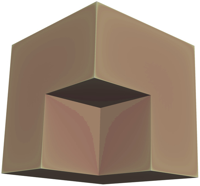
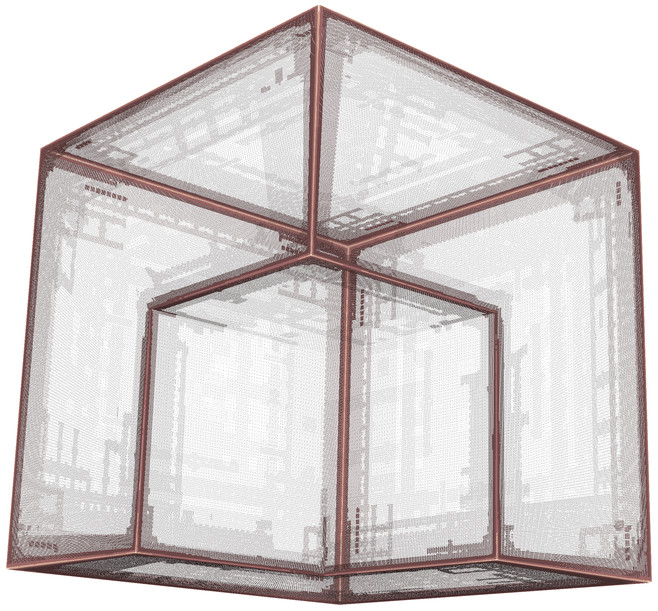
As a further example, we consider the solution of a scattering problem. Given an incident wave \(u_i\) and an obstacle \(\Omega\in\mathbb{R}^3\), we seek the scattered wave \(u_s\) such that total wave \(u = u_i+u_s\) satisfies the Helmholtz equation: \[ \begin{aligned} \Delta u + \kappa^2 u &= 0&&\text{in}\ \mathbb{R}^3\setminus\overline{\Omega},\\ u &= 0&&\text{on}\ \Gamma := \partial\Omega,\\ \lim_{r\to\infty} r \left\{ \frac{\partial u_s}{\partial r} - i\kappa u_s\right\} &= 0&&\text{as}\ r = \|{\bf x}\| \to\infty. \end{aligned} \] By using a linear combination of the acoustic double layer operator \(K\) and the acoustic single layer operator \(V\), the unknown Neumann datum \(\partial u/ \partial {\bf n}\) of the total field is obtain by a Fredholm integral equation of the second kind: \[ \bigg(\frac{1}{2}I+K-i\kappa V\bigg)^\top \frac{\partial u}{\partial {\bf n}} = \frac{\partial u_i}{\partial {\bf n}} -i\kappa u_i. \] A visualization of the mesh refinement and of the total wave \(u\) in case of a drilled cube is as follows:
Selected Publications
-
W. Dahmen, H. Harbrecht, and R. Schneider.
Adaptive methods for boundary integral equations. Complexity and
convergence estimates.
Math. Comput., 76(259):1243-1274, 2007.
-
T. Gantumur, H. Harbrecht, and R. Stevenson.
An optimal adaptive wavelet method without coarsening of the iterands.
Math. Comput.,
76(258):615-629, 2007.
-
H. Harbrecht, and M. Utzinger.
On adaptive wavelet boundary element methods.
J. Comput. Math., 36(1):90-109, 2018.