
Shape Optimization
Problem Formulation
Optimal shape design has become more and more important in engineering applications. Many problems that arise in structural mechanics, fluid dynamics and electromagnetics lead to the minimization of functionals, defined over a class of admissible domains and governed by the solutions of boundary value problems or initial boundary value problems.Mathematically speaking, one is interested in solving a minimization problem with respect to an unknown domain \[ J(\Omega) = \int_\Omega j\big({\bf x},u({\bf x}),\nabla u({\bf x})\big)\operatorname{d}\!{\bf x} \to \min, \] where the state function \(u\) solves the so-called state equation \begin{alignat*}{3} \mathcal{L}u &= f&&\quad\text{in}\ \Omega,\\ \mathcal{B}u &= g&&\quad\text{on}\ \Gamma. \end{alignat*} Additional constraints might be given with respect to the domain \(\Omega\) and its boundary \(\Gamma\): \begin{alignat*}{3} C_i(\Omega) &= \int_\Omega h_i({\bf x})\operatorname{d}\!{\bf x}\le c_i,&&\quad i=1,2,\dots,m,\\ C_i(\Gamma) &= \int_\Gamma h_i({\bf x})\operatorname{d}\!{\bf x}\le c_i,&&\quad i=m+1,m+2,\dots,n. \end{alignat*}
Numerical Solution of Shape Optimization Problems
In cooperation with Karsten Eppler (Dresden University of Technology, Germany), we are developing first and second order methods to solve such problems. Employing boundary variations by smooth fields \({\bf V}:\Gamma\to\mathbb{R}^n\), the shape gradient as well as the shape Hessian live only on the boundary \(\Gamma\) of the sought domain \(\Omega\). Boundary integral equations provide a rather efficient tool to compute the required data of the state function and the local shape derivatives. These boundary integral equations are solved by our wavelet Galerkin scheme which produces approximate solutions within a complexity that stays proportional to the number of boundary elements.An Example from Electromagnetic Shaping
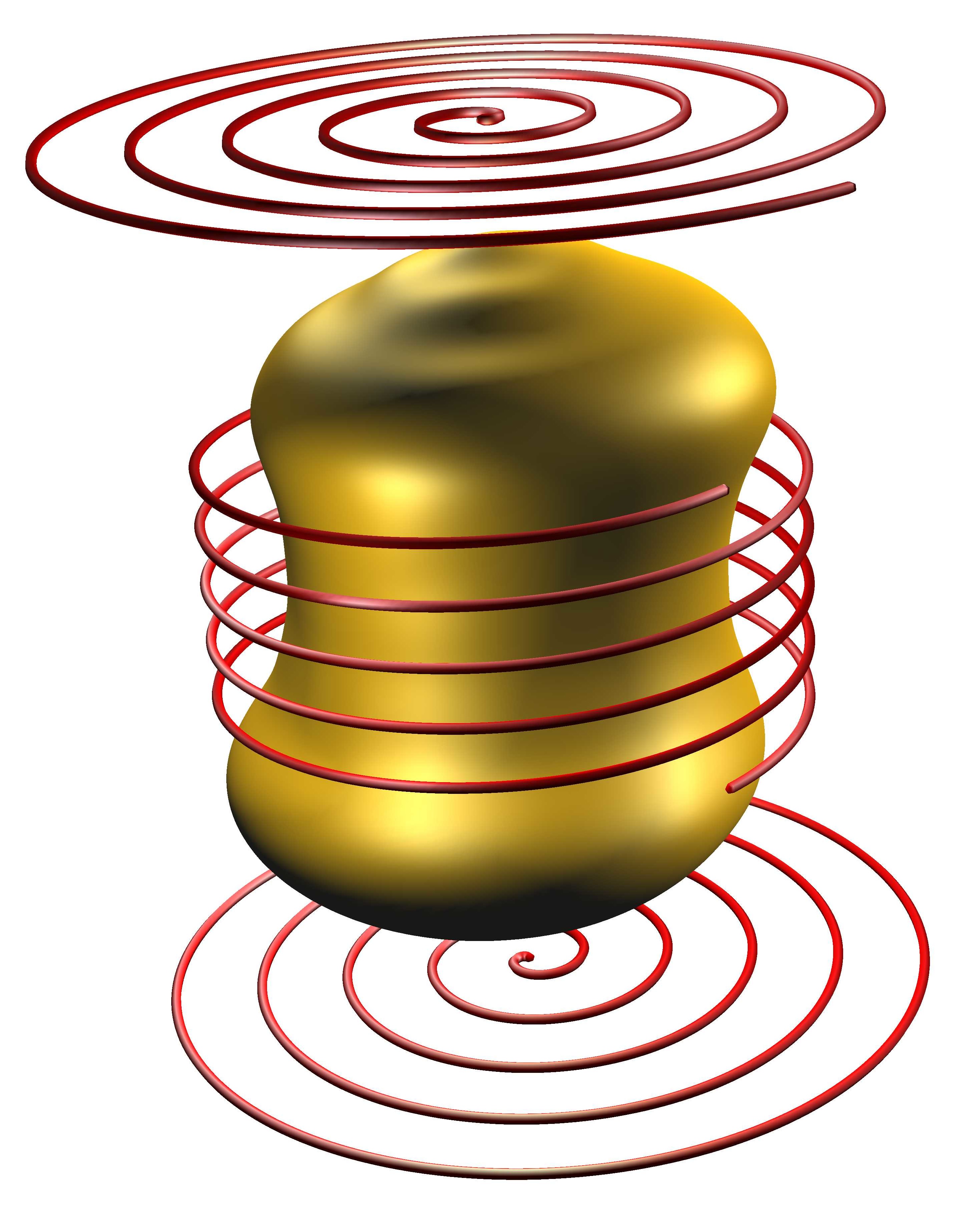
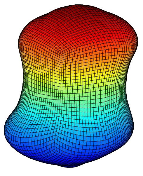
We consider a droplet \(\Omega\in\mathbb{R}^3\) of liquid metal levitating in a magnetic field generated by powered conductors, as shown in the subsequent figure.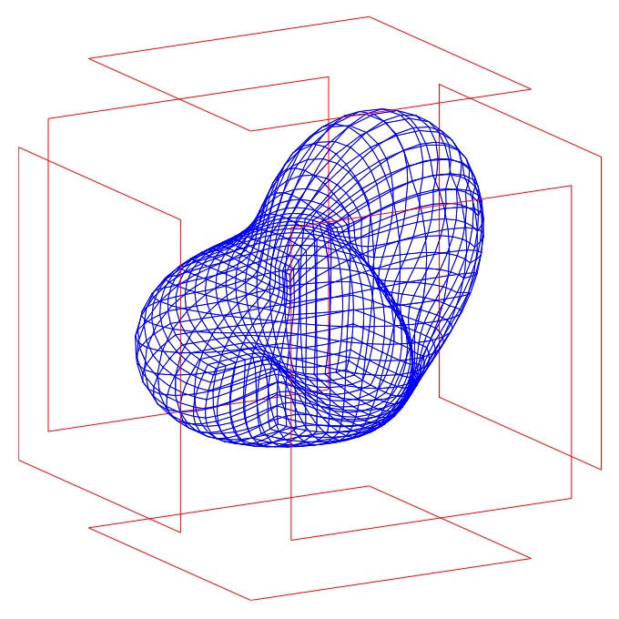
The shape of the droplet in the equilibrium can be computed by solving the following shape optimization problem: Find the domain \(\Omega\) such that \[ J(\Omega) = A \int_\Gamma 1 \operatorname{d}\!\sigma + B \int_\Omega x_3 \operatorname{d}\!{\bf x} - \int_{\Omega^c}\Vert{\bf B}\Vert{}^2\operatorname{d}\!{\bf x}\to\min, \] where the vector field \({\bf B}\) satisfies the magnetostatic Maxwell equations \begin{alignat*}{3} \nabla\times{\bf B} &= \mu_0 {\bf j}&&\quad\text{in}\ \Omega^c,\\ \operatorname{div}{\bf B} &= \mu_0&&\quad\text{in}\ \Omega^c,\\ \langle {\bf B},{\bf n}\rangle &= 0&&\quad\text{on}\ \Gamma,\\ \Vert{\bf B}\Vert &= \mathcal{O}(\Vert{\bf x}\Vert{}^{-1})&&\quad\text{as}\ \Vert{\bf x}\Vert\to\infty, \end{alignat*} subject to \(\vert\Omega\vert = V_0\). The shape gradient of the functional under consideration reads as \[ \delta J(\Omega)[{\bf V}] = \int_\Gamma \langle{\bf V},{\bf n}\rangle \big\{2A\mathcal{H} + Bx_3 + \Vert{\bf B}\Vert{}^2\big\}\operatorname{d}\!\sigma. \] For example, the simulation yields the following droplet in case of spiral wires:
Selected Publications
-
K. Eppler, H. Harbrecht, and R. Schneider.
On convergence in elliptic shape optimization.
SIAM J. Control Optim, 45:61-83, 2007.
-
K. Eppler and H. Harbrecht.
Wavelet based boundary element methods for exterior electromagnetic shaping.
Eng. Anal. Bound. Elem., 32(8):645-657, 2008.
-
H. Harbrecht.
Analytical and numerical methods in shape optimization.
Math. Methods Appl. Sci.,
31(18):2095-2114, 2008.
-
K. Eppler and H. Harbrecht.
Shape optimization for free boundary problems. Analysis and numerics.
In G. Leugering et al., editors, Constrained Optimization and Optimal Control for Partial Differential Equations,
volume 160 of International Series of Numerical Mathematics,
pages 277-288, Basel, 2012. Birkhäuser.