
Bernoulli Type Free Boundary Problems
Free boundary problems appear in many applications such as fluid dynamics, optimal design, electromagnetics and various other engineering fields. They deal with solving partial differential equations in a domain, a part of whose boundary is unknown in advance; that portion of the boundary is called a free boundary. Beside the standard boundary conditions that are needed in order to solve the partial differential equation, an additional condition must be imposed at the free boundary.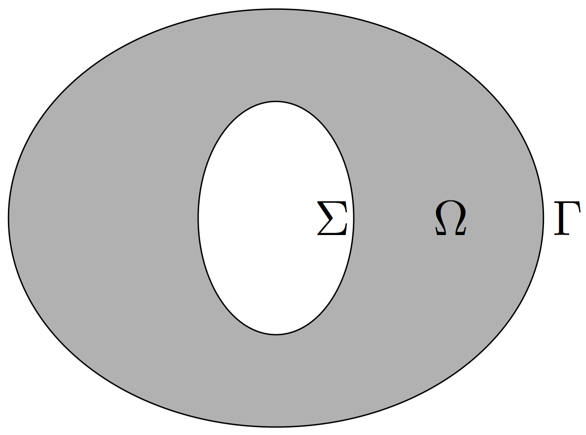
Consider an annular domain \(\Omega\) with interior, fixed boundary \(\Sigma\) and exterior, free boundary \(\Gamma\), as seen in the figure above. The Bernoulli type free boundary problem consists now in finding the free boundary \(\Gamma\) and an associated function \(u\in H^1(\Omega)\) such that the following overdetermined problem is satisfied: \[ \begin{aligned} -\Delta u &= f&&\qquad \text{in}\ \Omega,\\ u &= g&&\qquad \text{on}\ \Sigma,\\ -\frac{\partial u}{\partial {\bf n}} = h,& \quad u = 0 &&\qquad\text{on}\ \Gamma. \end{aligned} \] Here, \(f\ge 0\) and \(g,h>0\) are smooth functions where the sign conditions ensure that \(u\) is positive on \(\Omega\). For example, the growth of anodes in electrochemical processes is modeled by \(f \equiv 0\), \(g \equiv 1\), and \(h\equiv const\). Note that this choice corresponds to the original Bernoulli free boundary problem (named after Daniel Bernoulli, 1700-1782).
There are basically two approaches to compute the solution of free boundary problems. The free boundary problem can be reformulated as a shape optimization problem which is then solved by a gradient based optimization method. Alternatively, the trial method can be used, which is a fixed point iteration for the sought free boundary. Our research focusses on both approaches, especially on second order convergent algorithms.
The following figures show the resulting free boundaries for different choices of data in the case of a U-shape (left), an L-shape (middle), and four spheres (right) as interior domain:
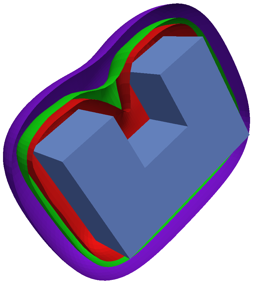

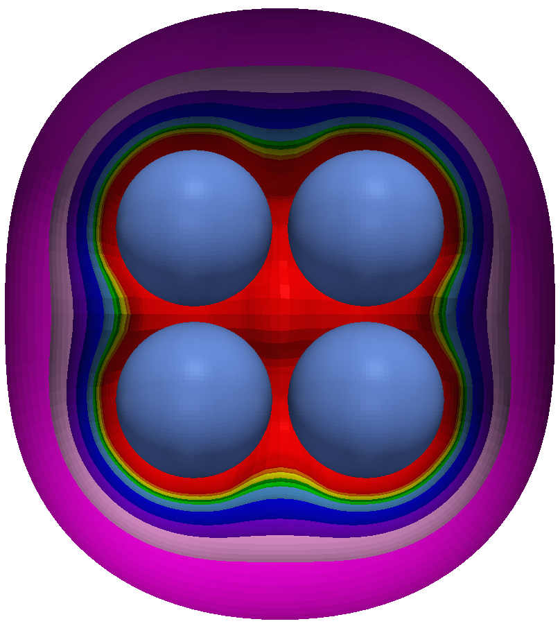
For the computation of these free boundaries, we used a second order convergent trial method. Starting with a sphere as initial free boundary, the current free boundary is updated in each step of the trial method according to an appropriate update rule. This process is repeated until it becomes stationary. An animation of the iterative solution process for the four spheres is found below.
Selected Publications
-
H. Harbrecht.
A Newton method for Bernoulli's free boundary problem in three
dimensions.
Computing, 82(1):11-30, 2008.
-
K. Eppler and H. Harbrecht.
Shape optimization for free boundary problems. Analysis and numerics.
In G. Leugering et al., editors, Constrained Optimization and Optimal Control for Partial Differential Equations,
volume 160 of International Series of Numerical Mathematics,
pages 277-288, Basel, 2012. Birkhäuser.
-
M. Bugeanu and H. Harbrecht.
A second order convergent trial method for free boundary problems in three dimensions.
Interfaces Free Bound., 17(4):517-537, 2015.